OVER Clause Overview
Let’s take a look at AdventureWorks Sales Order data in the United States (which is represented by TerritoryID’s 1 thru 5):
select sod.SalesOrderIDThanks to the OVER clause, we can effortlessly incorporate a column into that query that shows us each ProductID’s Average UnitPrice in that result:
,CustomerID
,ProductID
,UnitPrice
from AdventureWorks.Sales.SalesOrderDetail sod
join AdventureWorks.Sales.SalesOrderHeader soh on sod.SalesOrderID=soh.SalesOrderID
where TerritoryID between 1 and 5
order by SalesOrderID
,ProductID
/*
SalesOrderID CustomerID ProductID UnitPrice
------------ ---------- --------- ---------
43659 676 709 5.70
43659 676 711 20.1865
43659 676 712 5.1865
43659 676 714 28.8404
43659 676 716 28.8404
43659 676 771 2039.994
43659 676 772 2039.994
...
(60153 Rows Total)
*/
select sod.SalesOrderIDLet’s add one additional column that shows the UnitPrice’s Percent of the Average:
,CustomerID
,ProductID
,UnitPrice
,AvgPrice=avg(UnitPrice) over (partition by ProductID)
from AdventureWorks.Sales.SalesOrderDetail sod
join AdventureWorks.Sales.SalesOrderHeader soh on sod.SalesOrderID=soh.SalesOrderID
where TerritoryID between 1 and 5
order by SalesOrderID
,ProductID
/*
SalesOrderID CustomerID ProductID UnitPrice AvgPrice
------------ ---------- --------- --------- ---------
43659 676 709 5.70 5.6525
43659 676 711 20.1865 28.2153
43659 676 712 5.1865 7.0082
43659 676 714 28.8404 34.4369
43659 676 716 28.8404 35.1093
43659 676 771 2039.994 2085.9938
43659 676 772 2039.994 2043.917
...
(60153 Rows Total)
*/
select sod.SalesOrderIDAnd finally, let’s just look at the 50 Line Items that had the lowest Percentages by changing our ORDER BY and adding a TOP 50 to the query:
,CustomerID
,ProductID
,UnitPrice
,AvgPrice=avg(UnitPrice) over (partition by ProductID)
,PercentOfAvg=UnitPrice/avg(UnitPrice) over (partition by ProductID)*100
from AdventureWorks.Sales.SalesOrderDetail sod
join AdventureWorks.Sales.SalesOrderHeader soh on sod.SalesOrderID=soh.SalesOrderID
where TerritoryID between 1 and 5
order by SalesOrderID
,ProductID
/*
SalesOrderID CustomerID ProductID UnitPrice AvgPrice PercentOfAvg
------------ ---------- --------- --------- --------- ------------
43659 676 709 5.70 5.6525 100.84
43659 676 711 20.1865 28.2153 71.54
43659 676 712 5.1865 7.0082 74.00
43659 676 714 28.8404 34.4369 83.74
43659 676 716 28.8404 35.1093 82.14
43659 676 771 2039.994 2085.9938 97.79
43659 676 772 2039.994 2043.917 99.80
...
(60153 Rows Total)
*/
selectWell, that was easy. The OVER clause made our code nice and compact. If we didn’t have the OVER clause available to us, we would have had to write the query like the one below, JOINing our source data to a derived table where we computed the aggregate via a GROUP BY clause:
top 50 sod.SalesOrderID
,CustomerID
,ProductID
,UnitPrice
,AvgPrice=avg(UnitPrice) over (partition by ProductID)
,PercentOfAvg=UnitPrice/avg(UnitPrice) over (partition by ProductID)*100
from AdventureWorks.Sales.SalesOrderDetail sod
join AdventureWorks.Sales.SalesOrderHeader soh on sod.SalesOrderID=soh.SalesOrderID
where TerritoryID between 1 and 5
order by PercentOfAvg
,SalesOrderID
,ProductID
/*
SalesOrderID CustomerID ProductID UnitPrice AvgPrice PercentOfAvg
------------ ---------- --------- --------- -------- ------------
69408 236 987 112.998 337.3797 33.49
69413 43 987 112.998 337.3797 33.49
69418 381 987 112.998 337.3797 33.49
69442 233 987 112.998 337.3797 33.49
...
69418 381 984 112.998 330.3681 34.20
69422 650 984 112.998 330.3681 34.20
69452 9 984 112.998 330.3681 34.20
69468 237 984 112.998 330.3681 34.20
(50 Rows Total)
*/
;with SourceData asThat JOIN/GROUP BY approach took a lot more code and it looks like a lot of work, mainly because it has to scan the SalesOrderHeader and SalesOrderDetail tables twice, as we can see in the query plan:
(
select sod.SalesOrderID
,CustomerID
,ProductID
,UnitPrice
from AdventureWorks.Sales.SalesOrderDetail sod
join AdventureWorks.Sales.SalesOrderHeader soh on sod.SalesOrderID=soh.SalesOrderID
where soh.TerritoryID between 1 and 5
)
select
top 50 SalesOrderID
,CustomerID
,S.ProductID
,UnitPrice
,AvgPrice
,PercentOfAvg=UnitPrice/AvgPrice*100
from SourceData S
join (select ProductID
,AvgPrice=avg(UnitPrice)
from SourceData
group by ProductID) G on S.ProductID=G.ProductID
order by PercentOfAvg
,SalesOrderID
,ProductID
/*
SalesOrderID CustomerID ProductID UnitPrice AvgPrice PercentOfAvg
------------ ---------- --------- --------- -------- ------------
69408 236 987 112.998 337.3797 33.49
69413 43 987 112.998 337.3797 33.49
69418 381 987 112.998 337.3797 33.49
69442 233 987 112.998 337.3797 33.49
...
69418 381 984 112.998 330.3681 34.20
69422 650 984 112.998 330.3681 34.20
69452 9 984 112.998 330.3681 34.20
69468 237 984 112.998 330.3681 34.20
(50 Rows Total)
*/

The query plan of the OVER Clause query, on the other hand, only scans those tables once:

So it must be a lot more efficient, right?
Wrong.
Let’s take a look at the statistics for the two queries, collected by Profiler (with Query Results Discarded so that we are purely looking at processing time of the query and not the time to render the output):
/*
Description           Reads  Writes   CPU  Duration
---------------------------------------------------
OVER Clause          125801       2   617      1406
JOIN with GROUP BY     3916       0   308      1176
*/
The OVER clause was a real pig as far as the Number of Reads is concerned. And it had higher CPU and Duration than the JOIN approach.The OVER Clause Query Plan In Depth
Let’s take a closer look at the OVER clause actual execution plan once more, where I’ve added some annotations (please click on the image below to see a larger version in another browser window):

Looking at the outer loop (operators #5 thru #10), the rows that come from the merged table scans (#8, #9, #10) get sorted (#7) by ProductID. The Segment operator (#6) receives those rows and feeds them, groups (or segments) at a time, to the Table Spool operator (#5).
As the Table Spool (#5) receives those rows in a group, it saves a copy of the rows and then sends a single row to the Nested Loops operator (#4), indicating that it has done its job of saving the group’s rows.
Now that the Nested Loops operator (#4) has received its outer input, it calls for the inner input, which will come from operators #11 thru #15. The two other table spools in the plan (#14 and #15) are the same spool as #5, but they are replaying the copies of the rows that #5 had saved. The Stream Aggregate (#13) calculates the SUM(UnitPrice) and COUNT(*) and the Compute Scalar (#12) divides those two values to come up with the AVG(UnitPrice). This single value is JOINed (via the #11 Nested Loops operator) with the rows replayed by the Spool #15.
And then the Spool (#5) truncates its saved data and gets to work on the next group that it receives from the Segment operator (#6). And so on and so on, for each fresh group of ProductID's.
So, in a logical sense, this plan is also doing a GROUP BY and a JOIN, except it’s doing it with a single scan of the source data. However, to accomplish that, it has to do a triple scan of the spooled data, thus producing those hundreds of thousands of reads.
Memory Usage
If you hover your mouse over the SELECT operator (#1) in the actual query plan of our OVER Clause query, you can see that it requests a Memory Grant of 5288 Kbytes:

By comparison, our traditional JOIN/GROUP BY query only requests 1544 Kbytes.
In the case of the JOIN/GROUP BY query, the memory grant is for the “Top N” Sort and the two Hashing operators. As Adam Haines demonstrated in a recent blog entry, a TOP value of 100 or less does not require that much memory. It would only request 1024K. The additional memory required for the Hashes brought its request up to 1544K.
The OVER query, though is a different story. It also does a “Top N” Sort (#2), but, in addition, it does a full Sort (#7) of the source data, which requires a lot more memory than a “Top N” Sort. Thus the much larger memory grant request.
Things get a lot worse as we increase the size of our result set. Let’s add a lot more columns to our output, increasing the row size that the Sort operator must process from 27 bytes to 402 bytes…
selectFor this, the Memory Grant request balloons to 25,264K. If we add all those extra columns to our traditional JOIN/GROUP BY query, its Memory Grant request still remains at 1544K.
top 50 sod.SalesOrderID
,CustomerID
,ProductID
,UnitPrice
,AvgPrice=avg(UnitPrice) over (partition by ProductID)
,PercentOfAvg=UnitPrice/avg(UnitPrice) over (partition by ProductID)*100
/* Let's add a bunch of other columns */
,soh.AccountNumber,soh.BillToAddressID,soh.Comment,soh.ContactID
,soh.CreditCardApprovalCode,soh.CreditCardID,soh.CurrencyRateID,soh.DueDate
,soh.Freight,soh.ModifiedDate,soh.OnlineOrderFlag,soh.OrderDate
,soh.PurchaseOrderNumber,soh.RevisionNumber,soh.rowguid,soh.SalesOrderNumber
,soh.SalesPersonID,soh.ShipDate,soh.ShipMethodID,soh.ShipToAddressID
,soh.SubTotal,soh.TaxAmt,soh.TerritoryID,soh.TotalDue,sod.CarrierTrackingNumber
,sod.OrderQty,sod.SalesOrderDetailID,sod.SpecialOfferID,sod.UnitPriceDiscount
from AdventureWorks.Sales.SalesOrderDetail sod
join AdventureWorks.Sales.SalesOrderHeader soh on sod.SalesOrderID=soh.SalesOrderID
where TerritoryID between 1 and 5
order by PercentOfAvg
,SalesOrderID
,ProductID
Collecting Profiler statistics for the two queries with all those extra columns shows more interesting information:
/*
Description           Reads  Writes   CPU  Duration
---------------------------------------------------
OVER Clause          144936     790  1696      2125
JOIN with GROUP BY     3916       0   850      1725
*/
Note all the extra writes that were required for the OVER query. The row size of the data that we needed to sort is too big to do completely in memory and it spilled over into TempDB, writing 790 pages worth of data.The lesson here is that the JOIN/GROUP BY approach is faster and more efficient and less of a memory hog if you’re processing a large number of rows and/or if your rows are wide.
For our JOIN/GROUP BY query, the optimizer has the flexibility to choose from a variety of plans to come up with the most cost-effective approach. In our examples, the optimizer determined that it was more cost-effective to use a Hash Aggregation and a Hash Join as opposed to sorting the data. The Hash operators are extremely efficient in handling large gobs of data… and that data does not have to be sorted. The OVER query, on the other hand, requires the data to be sorted, because it always uses a Segment operator (#6) and a Stream Aggregate operator (#13) which only work on pre-sorted data.
Taking the SORT out of the Equation
Okay, so let’s do another experiment. Let’s see how our two approaches work on data that is pre-sorted. Just for kicks, instead of PARTITIONing BY (or GROUPing BY) ProductID, let’s do it by SalesOrderID. Since both the SalesOrderHeader and SalesOrderDetail tables have a clustered index on SalesOrderID, the system can scan both files in SalesOrderID order, and do Merge Joins to join the two tables together, and we won’t require any sorts at all. And let’s also take out our TOP 50 (and the ORDER BY) so that no “Top N” Sort has to be performed on either query. So we won’t require any memory grants at all in either query, and no expensive Sort operations. Here are the revised queries:
/* OVER Approach */Now let’s compare the performance of those two approaches:
select sod.SalesOrderID
,CustomerID
,ProductID
,UnitPrice
/* Let's add a bunch of other columns */
,soh.AccountNumber,soh.BillToAddressID,soh.Comment,soh.ContactID
,soh.CreditCardApprovalCode,soh.CreditCardID,soh.CurrencyRateID,soh.DueDate
,soh.Freight,soh.ModifiedDate,soh.OnlineOrderFlag,soh.OrderDate
,soh.PurchaseOrderNumber,soh.RevisionNumber,soh.rowguid,soh.SalesOrderNumber
,soh.SalesPersonID,soh.ShipDate,soh.ShipMethodID,soh.ShipToAddressID
,soh.SubTotal,soh.TaxAmt,soh.TerritoryID,soh.TotalDue,sod.CarrierTrackingNumber
,sod.OrderQty,sod.SalesOrderDetailID,sod.SpecialOfferID,sod.UnitPriceDiscount
,AvgPrice=avg(UnitPrice) over (partition by sod.SalesOrderID)
from AdventureWorks.Sales.SalesOrderDetail sod
join AdventureWorks.Sales.SalesOrderHeader soh on sod.SalesOrderID=soh.SalesOrderID
where TerritoryID between 1 and 5
/* JOIN/GROUP BY Approach */
;with SourceData as
(
select sod.SalesOrderID
,CustomerID
,ProductID
,UnitPrice
/* Let's add a bunch of other columns */
,soh.AccountNumber,soh.BillToAddressID,soh.Comment,soh.ContactID
,soh.CreditCardApprovalCode,soh.CreditCardID,soh.CurrencyRateID,soh.DueDate
,soh.Freight,soh.ModifiedDate,soh.OnlineOrderFlag,soh.OrderDate
,soh.PurchaseOrderNumber,soh.RevisionNumber,soh.rowguid,soh.SalesOrderNumber
,soh.SalesPersonID,soh.ShipDate,soh.ShipMethodID,soh.ShipToAddressID
,soh.SubTotal,soh.TaxAmt,soh.TerritoryID,soh.TotalDue,sod.CarrierTrackingNumber
,sod.OrderQty,sod.SalesOrderDetailID,sod.SpecialOfferID,sod.UnitPriceDiscount
from AdventureWorks.Sales.SalesOrderDetail sod
join AdventureWorks.Sales.SalesOrderHeader soh on sod.SalesOrderID=soh.SalesOrderID
where soh.TerritoryID between 1 and 5
)
select S.*
,AvgPrice
from SourceData S
join (select SalesOrderID
,AvgPrice=avg(UnitPrice)
from SourceData S
group by SalesOrderID) G on S.SalesOrderID=G.SalesOrderID
/*
Description           Reads  Writes   CPU  Duration
---------------------------------------------------
OVER Clause          192017       0  1445      1945
JOIN with GROUP BY     3914       0   683      1184
*/
The JOIN/GROUP BY query still outperforms the OVER query in every respect. The OVER query still had to do truckloads of Reads, because of the Spooling. Note that the reads this time were even higher than they were in our original example, because there are more Groups of SalesOrderID’s (12041) than there are Groups of ProductID’s (265), so the Spools worked overtime, saving and replaying all those extra groups of data.So it seems that the OVER clause is very convenient as far as coding and clarity, but unless you have pre-sorted data in a small number of groups with a small number of rows, the JOIN/GROUP BY approach may very well provide a better plan. That’s something to think about.
If you want the most efficient query possible, check out both approaches for performance. There may be some times when the optimizer will look at a JOIN/GROUP BY query and will construct a plan that is exactly like the OVER query anyway. For example, the following JOIN/GROUP BY query will do just that:
;with SourceData asInterestingly enough, it ONLY creates an OVER-type plan for the above because I specified that I wanted the output to be ORDERed BY ProductID, which is our GROUP BY column. Because of that, the optimizer figured it was more cost-effective to SORT the data by ProductID up front and do the spooling stuff than it was to do the Hashing approach and SORT the final data by ProductID at the end. If you take the ORDER BY out of the query above, then the optimizer will revert back to a plan with Hash operators and no spooling.
(
select sod.SalesOrderID
,CustomerID
,ProductID
,UnitPrice
from AdventureWorks.Sales.SalesOrderDetail sod
join AdventureWorks.Sales.SalesOrderHeader soh on sod.SalesOrderID=soh.SalesOrderID
where soh.TerritoryID between 1 and 5
)
select SalesOrderID
,CustomerID
,S.ProductID
,UnitPrice
,AvgPrice
,PercentOfAvg=UnitPrice/AvgPrice*100
from SourceData S
join (select ProductID
,AvgPrice=avg(UnitPrice)
from SourceData
group by ProductID) G on S.ProductID=G.ProductID
order by ProductID
But I DISTINCTly Asked For…
I know I’ve kind of trashed the OVER clause a bit during the course of this article, and I hate to kick someone when they’re down, but I’m afraid I have to bring something else up.
The OVER clause does not accept DISTINCT in its aggregate functions. In other words, the following query will bring about an error:
select SalesOrderIDIf you want DISTINCT aggregates, you are forced to use the JOIN/GROUP BY approach to accomplish this.
,ProductID
,UnitPrice
,NumDistinctPrices=count(distinct UnitPrice) over (partition by ProductID)
,AvgDistinctPrice=avg(distinct UnitPrice) over (partition by ProductID)
from AdventureWorks.Sales.SalesOrderDetail
/*
Msg 102, Level 15, State 1, Line 4
Incorrect syntax near 'distinct'.
*/
However, there may be times when, for whatever reason, you must scan the data only once. To be honest, the whole catalyst for my writing this article was a situation just like that. My source data was a derived table that produced random rows… something like this:
;with RandomRowNumsAdded as(If you’re wondering why the heck I’d want something like this, then stay tuned… you’ll see why in a future blog post… my craziest one yet).
(
select SalesOrderID
,ProductID
,UnitPrice
,RowNum=row_number() over (order by newid())
from AdventureWorks.Sales.SalesOrderDetail
)
select SalesOrderID
,ProductID
,UnitPrice
from RandomRowNumsAdded
where RowNum<=50
/*
SalesOrderID ProductID UnitPrice
------------ --------- ----------
47439 762 469.794
72888 873 2.29
47640 780 2071.4196
51143 883 31.3142
. . .
48393 798 600.2625
63980 711 34.99
64590 780 2319.99
64262 877 7.95
(50 Rows Total)
*/
Clearly, that query will come out differently every time it is executed, so if I wanted to use a JOIN/GROUP BY to calculate a COUNT(DISTINCT) or AVG(DISTINCT), I couldn’t, because by scanning the information twice, each scan would produce two different outcomes and therefore the following JOIN/GROUP BY approach would not work, because the two scans would produce two different sets of ProductID’s and UnitPrices:
;with RandomRowNumsAdded asSo I had to come up with a different way to do DISTINCT aggregates by only doing a single scan on the source data.
(
select SalesOrderID
,ProductID
,UnitPrice
,RowNum=row_number() over (order by newid())
from AdventureWorks.Sales.SalesOrderDetail
)
,SourceData as
(
select SalesOrderID
,ProductID
,UnitPrice
from RandomRowNumsAdded
where RowNum<=50
)
select S.*
,NumDistinctPrices
,AvgDistinctPrice
from SourceData S
join (select ProductID
,NumDistinctPrices=count(distinct UnitPrice)
,AvgDistinctPrice=avg(distinct UnitPrice)
from SourceData
group by ProductID) G on S.ProductID=G.ProductID
/*
Because of the two SCANs of the data, the JOIN above will
produce different numbers of rows (sometimes perhaps even
ZERO rows!) every time this query is run.
*/
The answer ended up being… ta-dah!... the OVER clause, ironically enough. Even though you can’t do DISTINCT Aggregates directly with OVER, you can accomplish the task by first performing a ranking function (ROW_NUMBER()), and then follow that with a traditional non-DISTINCT aggregation. Here’s how, using my random-row source data:
;with RandomRowNumsAdded asWe use ROW_NUMBER() to introduce a PriceSeq column, which resets to a value of 1 for each ProductID and UnitPrice combination. And then we only aggregate on those UnitPrices that have a PriceSeq of 1, since any rows with a PriceSeq of 2 and above will just be duplicate (non-DISTINCT) repeats of a ProductID and UnitPrice combination.
(
select SalesOrderID
,ProductID
,UnitPrice
,RowNum=row_number() over (order by newid())
from AdventureWorks.Sales.SalesOrderDetail
)
,SourceData as
(
select SalesOrderID
,ProductID
,UnitPrice
,PriceSeq=row_number() over (partition by ProductID,UnitPrice order by UnitPrice)
from RandomRowNumsAdded
where RowNum<=50
)
select SalesOrderID
,ProductID
,UnitPrice
,NumDistinctPrices=count(case when PriceSeq=1 then UnitPrice end)
over (partition by ProductID)
,AvgDistinctPrice=avg(case when PriceSeq=1 then UnitPrice end)
over (partition by ProductID)
from SourceData
/*
SalesOrderID ProductID UnitPrice NumDistinctPrices AvgDistinctPrice
------------ --------- --------- ----------------- ----------------
73078 708 34.99 1 34.99
74332 708 34.99 1 34.99
69526 711 19.2445 2 27.1172
64795 711 34.99 2 27.1172
. . .
51810 940 48.594 1 48.594
68514 955 2384.07 1 2384.07
71835 964 445.41 1 445.41
51823 968 1430.442 1 1430.442
(50 Rows Total)
*/
We already saw how an OVER aggregation query requires a Sort. In order to calculate DISTINCT aggregations, we require two sorts… one for the ROW_NUMBER() function to calculate our PriceSeq column and a second to do the aggregation. You can see this in the query plan:

This is a little odd, because the first sort orders the data by ProductID and UnitPrice, and the second sort orders the data by just ProductID. But that second sort is not necessary, because the first sort already put the data in a ProductID order anyway. It seems that the optimizer is not “smart enough” to know this and take advantage of it.
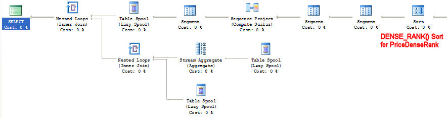
However, all is not completely lost. If the only DISTINCT aggregation you require in your query is a COUNT(), then you can use yet another clever approach to accomplish this:
;with RandomRowNumsAdded asThis applies a DENSE_RANK() value to each different UnitPrice found within each ProductID, and we can then calculate the COUNT(DISTINCT) by just getting the MAX() of that PriceDenseRank value.
(
select SalesOrderID
,ProductID
,UnitPrice
,RowNum=row_number() over (order by newid())
from AdventureWorks.Sales.SalesOrderDetail
)
,SourceData as
(
select SalesOrderID
,ProductID
,UnitPrice
,PriceDenseRank=dense_rank() over (partition by ProductID order by UnitPrice)
from RandomRowNumsAdded
where RowNum<=50
)
select SalesOrderID
,ProductID
,UnitPrice
,NumDistinctPrices=max(PriceDenseRank) over (partition by ProductID)
from SourceData
/*
SalesOrderID ProductID UnitPrice NumDistinctPrices
------------ --------- --------- -----------------
67354 707 34.99 1
51653 707 34.99 1
58908 708 20.994 2
66632 708 34.99 2
. . .
51140 975 1020.594 1
68191 976 1700.99 1
72706 984 564.99 1
53606 987 338.994 1
(50 Rows Total)
*/
Since the DENSE_RANK() and the MAX() both do a PARTITION BY ProductID, their sorting requirements are exactly identical, and this query plan only requires a single sort as opposed to two:
Final Wrapup
I hope you enjoyed this in-depth look at Aggregations and the OVER Clause. To review what was illustrated in this article…
- The OVER clause is very convenient for calculating aggregations, but using a JOIN/GROUP BY approach may very well perform more efficiently, especially on source data that has a large number of rows and/or has a wide row size and/or is unsorted.
- If you want to calculate DISTINCT Aggregates, use the JOIN/GROUP BY approach; however, …
- If you, for some reason, only want to scan the source data once, assign sequence numbers using ROW_NUMBER() and then aggregate only on those rows that received a sequence number of 1; however, …
- If you only require COUNT(DISTINCT), then use DENSE_RANK() and MAX(), since that only requires a single sort instead of two.


Thanx Brad.
ReplyDeleteI'm currently working on a mega-query that get data, aggregates on four different levels, then pulls them all together for calculations. I kept thinking that i could give it a workOVER() and mash it all together. I figured it'd be a killer on the performance. The one read is nice, but the price, oh the price...
I also wanted to use ROLLUP for the aggregations. It also takes a lot longer. Somewhere around 150% of the base query time, in a quick test in my mega-query.
I'm finding most of the features in SQL Server are added convenience as the cost of processing time. It makes me wonder why they added them at all.
I used this post for work today. Thought you'd like to know.
ReplyDelete@Brian:
ReplyDeleteI understand what you're saying... I really like the features added to the product... they can certainly be very helpful, but one shouldn't use them blindly.
@Michael:
Cool... what specifically? One of the DISTINCT tricks? Or a JOIN/GROUPBY in lieu of the OVER?
Well to be honest, I've never used the OVER clause this way before. So I gave it a spin. What I like about it is the syntactical nice-ness.
ReplyDeleteLest you say "THAT WASN'T THE POINT OF THE ARTICLE" I did compare it to the GROUP BY subclause equivalent and my results were similar to your.
In a battle between nice syntax and nice performance, performance wins each time, it's just sad it has to be that way.
I agree with you completely about the "syntactical niceness"... I LIKE the OVER clause... really!
ReplyDeleteAnd even though the point of the article ended up being about its shortcomings, I didn't start it out that way. At first I just wanted to talk about the lack of its support for DISTINCT (and how to get around it), but then as I dug further and further, I found that it can have performance problems with large and/or wide data sources.
Thanks, as always, for the feedback.
--Brad