All I Want is a Normal(ized) Life

It looks like my blog’s theme for December is turning out to be Problem Databases.

My last blog entry talked about a database I was dealing with that consisted entirely of indecipherably-named heaps with multiple-column logical keys.

This time I have a database that is not normalized and has just plain bad data in it that’s got to be fixed. It was easy to fix, though, so this post is not rocket science, but I figured I’d do a quick write-up about it anyway.

Let me give you an example of what I was dealing with using data from good old AdventureWorks.

The following builds a temporary table consisting of the total sales grouped by Product, Customer, and SalesPerson. Only Products that are categorized as Clothing are used to populate the table, just to keep it relatively small for this example.

if object_id('tempdb..#ProdSalesInfo','U') is not null drop table #ProdSalesInfo
go 
select p.ProductID
      ,p.Name
      ,h.CustomerID
      ,h.SalesPersonID
      ,sum(d.LineTotal) as Dollars
into #ProdSalesInfo
from Production.Product p
join Production.ProductSubcategory c on p.ProductSubcategoryID=c.ProductSubcategoryID 
join Sales.SalesOrderDetail d on p.ProductID=d.ProductID
join Sales.SalesOrderHeader h on d.SalesOrderID=h.SalesOrderID 
where c.ProductCategoryID=3  /* Clothing Items */
  and h.SalesPersonID is not null
group by p.ProductID
        ,p.Name
        ,h.CustomerID
        ,h.SalesPersonID 
;
/*
(4716 row(s) affected)
*/

Notice that I included the Product’s Name in this table also. This was similar to the table that I was working with. There was no “master” table of Products… no table that I could JOIN with to acquire the Name of the Product… all the Product Names were only in this statistical table… duplicated over and over as you can see:

select *
from #ProdSalesInfo
order by ProductID
;
/*
ProductID Name                            CustomerID SalesPersonID    Dollars
--------- ------------------------------- ---------- ------------- ----------
      709 Mountain Bike Socks, M                  11           282  34.200000
      709 Mountain Bike Socks, M                  17           275 102.600000
      709 Mountain Bike Socks, M                  18           275  45.600000
      709 Mountain Bike Socks, M                  20           283 110.397600
      . . .
      857 Men's Bib-Shorts, L                    184           277 431.952000
      857 Men's Bib-Shorts, L                    197           275  53.994000
      857 Men's Bib-Shorts, L                    203           281 107.988000
      . . .      
      884 Short-Sleeve Classic Jersey, XL        688           290 323.940000
      884 Short-Sleeve Classic Jersey, XL        692           287 388.728000
      884 Short-Sleeve Classic Jersey, XL        695           275 485.910000
      884 Short-Sleeve Classic Jersey, XL        700           279 726.295076
(4716 rows total)      
*/

So, for example, there are 70 entries in the table for ProductID 709, and all of them have the same description duplicated over and over for each of those entries. We’re in Non-normalized Territory.

However, it was worse than this.

Most of the names for a given ProductID were consistent, but there were inconsistent names scattered here and there for most of the ProductIDs.

Let’s duplicate that situation by altering the names of a random 3% sampling of all the entries in the table:

with cte as
(
  select Name
        ,abs(checksum(newid()))%100 as RandUpTo100
  from #ProdSalesInfo
)
update cte
set Name=Name+'-JUNK'
where RandUpTo100<=3  /* 3% of the items */
;
/*
(174 row(s) affected)
*/

Now when we take a look at the table’s contents, we can see that there are junk names scattered randomly throughout (your results will differ):

select *
from #ProdSalesInfo
order by ProductID
;
/*
ProductID Name                                 CustomerID SalesPersonID    Dollars
--------- ------------------------------------ ---------- ------------- ----------
      709 Mountain Bike Socks, M-JUNK                  11           282  34.200000
      709 Mountain Bike Socks, M-JUNK                  17           275 102.600000
      709 Mountain Bike Socks, M                       18           275  45.600000
      709 Mountain Bike Socks, M                       20           283 110.397600
      . . .
      857 Men's Bib-Shorts, L                         184           277 431.952000
      857 Men's Bib-Shorts, L-JUNK                    197           275  53.994000
      857 Men's Bib-Shorts, L                         203           281 107.988000
      . . .      
      884 Short-Sleeve Classic Jersey, XL             688           290 323.940000
      884 Short-Sleeve Classic Jersey, XL-JUNK        692           287 388.728000
      884 Short-Sleeve Classic Jersey, XL             695           275 485.910000
      884 Short-Sleeve Classic Jersey, XL             700           279 726.295076
(4716 rows total)      
*/

A handful of the Products don’t have any inconsistent names at all, but rather have a uniform name for each of their entries:

select ProductID
from #ProdSalesInfo
group by ProductID
having count(distinct Name)=1
;
/*
ProductID
---------
      710
      866
*/

But most of the Products have more than one name:

select ProductID
from #ProdSalesInfo
group by ProductID
having count(distinct Name)>1
;
/*
ProductID
---------
      709
      712
      714
    . . .
      881
      883
      884
(30 rows total)      
*/

We want to fix the data in this table so that each of the Products has one and only one name. For any given ProductID, the name that has the most entries is the “master”… it is the “Good” Name… and all other names for the ProductID should be overwritten with that Good Name.

As I mentioned previously, this is easy to do, as long as you attack the problem one step at a time.

Let’s take a look at our problem Products (those with more than one name) and see how many entries there are for each of their names:

with ProblemProds as
(
  select ProductID
  from #ProdSalesInfo
  group by ProductID
  having count(distinct Name)>1
)
select ProductID
      ,Name
      ,count(*) as NumEntries
from #ProdSalesInfo
where ProductID in (select ProductID from ProblemProds)
group by ProductID
        ,Name
order by ProductID
        ,NumEntries desc
;       
/*
ProductID Name                                 NumEntries
--------- ------------------------------------ ----------
      709 Mountain Bike Socks, M                       69
      709 Mountain Bike Socks, M-JUNK                   4
      712 AWC Logo Cap                                337
      712 AWC Logo Cap-JUNK                            11
      714 Long-Sleeve Logo Jersey, M                  254
      714 Long-Sleeve Logo Jersey, M-JUNK               8
      . . .
      881 Short-Sleeve Classic Jersey, S              131
      881 Short-Sleeve Classic Jersey, S-JUNK           4
      883 Short-Sleeve Classic Jersey, L              173
      883 Short-Sleeve Classic Jersey, L-JUNK           9
      884 Short-Sleeve Classic Jersey, XL             177
      884 Short-Sleeve Classic Jersey, XL-JUNK          4
(60 rows total)
*/

I sorted the output by ProductID and then in descending order of NumEntries. This way the name with the most entries will be output first for each ProductID… those are our Good Names.

But how do we filter out those Good Names within a query?

It’s the good old Window Functions to the rescue. We can use the ROW_NUMBER() ranking function to assign a row number to our rows. For each ProductID (PARTITION BY ProductID), we want to assign a row number (starting with 1) to the rows in descending order of the number of entries for the Name (ORDER BY COUNT(*) DESC):

with ProblemProds as
(
  select ProductID
  from #ProdSalesInfo
  group by ProductID
  having count(distinct Name)>1
)
select ProductID
      ,Name
      ,count(*) as NumEntries
      ,row_number() over (partition by ProductID
                          order by count(*) desc) as RowNum
from #ProdSalesInfo
where ProductID in (select ProductID from ProblemProds)
group by ProductID
        ,Name
order by ProductID
        ,NumEntries desc
;
/*
ProductID Name                                 NumEntries RowNum
--------- ------------------------------------ ---------- ------
      709 Mountain Bike Socks, M                       69      1
      709 Mountain Bike Socks, M-JUNK                   4      2
      712 AWC Logo Cap                                337      1
      712 AWC Logo Cap-JUNK                            11      2
      714 Long-Sleeve Logo Jersey, M                  254      1
      714 Long-Sleeve Logo Jersey, M-JUNK               8      2
      . . .
      881 Short-Sleeve Classic Jersey, S              131      1
      881 Short-Sleeve Classic Jersey, S-JUNK           4      2
      883 Short-Sleeve Classic Jersey, L              173      1
      883 Short-Sleeve Classic Jersey, L-JUNK           9      2
      884 Short-Sleeve Classic Jersey, XL             177      1
      884 Short-Sleeve Classic Jersey, XL-JUNK          4      2
(60 rows total)
*/

By applying this ROW_NUMBER() ranking function to the query, we can see that all the rows with a value of 1 are the names with the most occurrences… those are our Good Names that we can use to overwrite all the Bad Names.

So here are our Good Names… the ones with a row number equal to 1:

with ProblemProds as
(
  select ProductID
  from #ProdSalesInfo
  group by ProductID
  having count(distinct Name)>1
)
,ProdNameSummary as
(
  select ProductID
        ,Name
        ,count(*) as NumEntries
        ,row_number() over (partition by ProductID
                            order by count(*) desc) as RowNum
  from #ProdSalesInfo
  where ProductID in (select ProductID from ProblemProds)
  group by ProductID
          ,Name
)
select ProductID
      ,Name as GoodName
from ProdNameSummary
where RowNum=1
;
/*
ProductID GoodName                           
--------- -------------------------------
      709 Mountain Bike Socks, M         
      712 AWC Logo Cap                   
      714 Long-Sleeve Logo Jersey, M     
      715 Long-Sleeve Logo Jersey, L     
      875 Racing Socks, L                
      881 Short-Sleeve Classic Jersey, S 
      883 Short-Sleeve Classic Jersey, L 
      884 Short-Sleeve Classic Jersey, XL
(30 rows total)
*/

Now that we have that set of “Good” Names, we can JOIN it back to our table in order to find all the entries that have the Bad Names… in other words, those entries whose Name is not equal to the Good Name.

with ProblemProds as
(
  select ProductID
  from #ProdSalesInfo
  group by ProductID
  having count(distinct Name)>1
)
,ProdNameSummary as
(
  select ProductID
        ,Name
        ,count(*) as NumEntries
        ,row_number() over (partition by ProductID
                            order by count(*) desc) as RowNum
  from #ProdSalesInfo
  where ProductID in (select ProductID from ProblemProds)
  group by ProductID
          ,Name
)
,GoodNames as
(
  select ProductID
        ,Name as GoodName
  from ProdNameSummary
  where RowNum=1
)
select p.ProductID
      ,p.Name as BadName
      ,c.GoodName
from #ProdSalesInfo p
join GoodNames c on p.ProductID=c.ProductID
where p.Name<>GoodName
order by p.ProductID
;
/*
ProductID BadName                              GoodName
--------- ------------------------------------ -------------------------------
      709 Mountain Bike Socks, M-JUNK          Mountain Bike Socks, M
      709 Mountain Bike Socks, M-JUNK          Mountain Bike Socks, M
      709 Mountain Bike Socks, M-JUNK          Mountain Bike Socks, M
      709 Mountain Bike Socks, M-JUNK          Mountain Bike Socks, M
      712 AWC Logo Cap-JUNK                    AWC Logo Cap
      712 AWC Logo Cap-JUNK                    AWC Logo Cap
      . . .
      883 Short-Sleeve Classic Jersey, L-JUNK  Short-Sleeve Classic Jersey, L
      883 Short-Sleeve Classic Jersey, L-JUNK  Short-Sleeve Classic Jersey, L
      884 Short-Sleeve Classic Jersey, XL-JUNK Short-Sleeve Classic Jersey, XL
      884 Short-Sleeve Classic Jersey, XL-JUNK Short-Sleeve Classic Jersey, XL
      884 Short-Sleeve Classic Jersey, XL-JUNK Short-Sleeve Classic Jersey, XL
      884 Short-Sleeve Classic Jersey, XL-JUNK Short-Sleeve Classic Jersey, XL
(176 rows total)      
*/

That’s our list of the entries with the Bad Names and the Good Name that we should use to overwrite them.

To be honest, though, it bugs me that the above query is scanning the table 3 times. There’s no compelling reason to use the ProblemProds CTE anymore. We could just perform the ROW_NUMBER() assignment to ALL products, whether they have Bad Names or not. Our two ProductIDs (710 and 866) that already have only 1 name still won’t be in the final output because the predicate of p.Name<>GoodName will filter them out anyway.

So let’s get rid of the ProblemProds CTE, and we’ll end up with the same output, but this time we will have only scanned our table 2 times instead of 3:

with ProdNameSummary as
(
  select ProductID
        ,Name
        ,count(*) as NumEntries
        ,row_number() over (partition by ProductID
                            order by count(*) desc) as RowNum
  from #ProdSalesInfo
  group by ProductID
          ,Name
)
,GoodNames as
(
  select ProductID
        ,Name as GoodName
  from ProdNameSummary
  where RowNum=1
)
select p.ProductID
      ,p.Name as BadName
      ,c.GoodName
from #ProdSalesInfo p
join GoodNames c on p.ProductID=c.ProductID
where p.Name<>GoodName
order by p.ProductID
;
/*
ProductID BadName                              GoodName
--------- ------------------------------------ -------------------------------
      709 Mountain Bike Socks, M-JUNK          Mountain Bike Socks, M
      709 Mountain Bike Socks, M-JUNK          Mountain Bike Socks, M
      709 Mountain Bike Socks, M-JUNK          Mountain Bike Socks, M
      709 Mountain Bike Socks, M-JUNK          Mountain Bike Socks, M
      712 AWC Logo Cap-JUNK                    AWC Logo Cap
      712 AWC Logo Cap-JUNK                    AWC Logo Cap
      . . .
      883 Short-Sleeve Classic Jersey, L-JUNK  Short-Sleeve Classic Jersey, L
      883 Short-Sleeve Classic Jersey, L-JUNK  Short-Sleeve Classic Jersey, L
      884 Short-Sleeve Classic Jersey, XL-JUNK Short-Sleeve Classic Jersey, XL
      884 Short-Sleeve Classic Jersey, XL-JUNK Short-Sleeve Classic Jersey, XL
      884 Short-Sleeve Classic Jersey, XL-JUNK Short-Sleeve Classic Jersey, XL
      884 Short-Sleeve Classic Jersey, XL-JUNK Short-Sleeve Classic Jersey, XL
(176 rows total)      
*/

So now it’s just a simple matter of commenting out the SELECT command (and the ORDER BY clause) and inserting an UPDATE command to fix those Bad Names:

with ProdNameSummary as
(
  select ProductID
        ,Name
        ,count(*) as NumEntries
        ,row_number() over (partition by ProductID
                            order by count(*) desc) as RowNum
  from #ProdSalesInfo
  group by ProductID
          ,Name
)
,GoodNames as
(
  select ProductID
        ,Name as GoodName
  from ProdNameSummary
  where RowNum=1
)
/*
select p.ProductID
      ,p.Name as BadName
      ,c.GoodName
*/
update p
set Name=c.GoodName
from #ProdSalesInfo p
join GoodNames c on p.ProductID=c.ProductID
where p.Name<>GoodName
/*
order by p.ProductID
*/
;
/*
(176 row(s) affected)
*/

And we’re done!

Let’s check our work to make sure that there are no ProductIDs with more than one Name:

select ProductID
from #ProdSalesInfo
group by ProductID
having count(distinct Name)>1
;
/*
Nothing... Nada... Zip... Empty
It's all good.
*/

Looks like it worked.

Now that the original data is fixed up, our final step is to do what should have been done long ago… Create a Product “master” table:

select distinct ProductID
               ,Name
into #ProdMaster
from #ProdSalesInfo
;
/*
(32 row(s) affected)
*/
alter table #ProdMaster add constraint PK_ProdMaster primary key (ProductID)

And then hunt down any code that relies on the Name column in #ProdSalesInfo… something like the following is a good start. If you’re wondering about the ObjDefLink column, please see my blog post called Hyperlinks To T-SQL Code for an explanation.

select ObjType=type_desc 
      ,ObjName=schema_name(schema_id)+'.'+name
      ,ObjDefLink
from sys.objects
cross apply (select ObjDef=object_definition(object_id)) F1
cross apply (select ObjDefLink=(select [processing-instruction(q)]=ObjDef
                                for xml path(''),type)) F2
where type in ('P'             /* Procedures */
              ,'V'             /* Views */
              ,'TR'            /* Triggers */
              ,'FN','IF','TF'  /* Functions */
              ) 
  and ObjDef like '%#ProdSalesInfo%' /* String to search for */ 
  and ObjDef like '%Name%'           /* Additional string to search for */
order by charindex('F',type) desc  /* Group the functions together */
        ,ObjType
        ,ObjName
 

And any external application code that does direct querying of the database and makes use of the #ProdSalesInfo.Name column would have to be sought out also.

Once we find all those, then we can phase out the use of the #ProdSalesInfo.Name column and instead use the Name column in our new #ProdMaster table via a JOIN.

Finally, we can sleep easier at night, knowing the database is in a more normalized state.

HEAPS o’ Trouble: A Follow-Up

Just wanted to give you all a heads-up in case any of missed it...

After reading my HEAPS o’ Trouble With Multiple JOINs blog post from a few days ago, Paul White (blog|twitter) wrote a follow-up to the post. I was really delighted with his article... it's an excellent must-read, giving some terrific additional insights into the optimizer.

If you’re not a regular reader of his blog, I must insist that you subscribe to it immediately. It’s a gold mine of terrific material. Consider it an early Christmas present that keeps giving all year long.

HEAPs o’ Trouble With Multi-Column JOINs

You would just love the database that I’m dealing with at a client site.

First of all, the database has impossible-to-decipher 5-character table names, and their column names are just as bad, so I’m dealing with objects with awful names that look like XQUMB.XUMHF and YRWNO.YWNVZ.

Second of all, every table in the database is a Heap with no primary keys or indexes defined at all.

Great, huh?

But wait… that’s not all!

There are no small simple surrogate keys to logically tie the tables together in any kind of a relationship. Many of the tables have a logical key made up of multiple columns. So when I look at the stored procedures that JOIN the tables together, I see ugly stuff like this:

select X.XUMHF
      ,X.XUMRO
      ,X.XUMBC
      ,X.XUMPU
      ,Y.YWNOQ
      ,B.BFUCP
      ,B.BFUVX
from XQUMB as X 
join YRWNO as Y on X.XUMHF=Y.YWNHF 
                and X.XUMRO=Y.YWNRO 
                and X.XUMBC=Y.YWNBC
join BRFUP as B on Y.YWNHF=B.BFUHF 
                and Y.YWNRO=B.BFURO 
                and Y.YWNBC=B.BFUBC 
                and Y.YWNCP=B.BFUCP
 

Doesn’t that look like fun?

None of the tables are really that large in terms of rows, so I figured performance would not be that big of a deal.

WRONG!

Bad assumption.

I’ve been so spoiled by only dealing with databases with well-defined keys and indexes that I never realized what a heap o’ trouble Heaps can be… especially when it comes to multi-column JOINs.

Let me illustrate with our old friend the AdventureWorks database.

Here’s a simple JOIN of 4 tables in the original database (with appropriate keys and indexes):

select p.ProductID as PID
      ,p.Name
      ,d.OrderQty
      ,h.SalesOrderNumber
      ,h.OrderDate
      ,c.TerritoryID
from AdventureWorks.Production.Product p
join AdventureWorks.Sales.SalesOrderDetail d on p.ProductID=d.ProductID
join AdventureWorks.Sales.SalesOrderHeader h on d.SalesOrderID=h.SalesOrderID
join AdventureWorks.Sales.Customer c on h.CustomerID=c.CustomerID 
order by p.ProductID
/*
PID Name                  OrderQty SalesOrderNumber OrderDate  TerritoryID
--- --------------------- -------- ---------------- ---------- -----------
707 Sport-100 Helmet, Red        1 SO43665          2001-07-01           1
707 Sport-100 Helmet, Red        2 SO43668          2001-07-01           6
707 Sport-100 Helmet, Red        4 SO43673          2001-07-01           2
. . .
999 Road-750 Black, 52           1 SO73926          2004-06-27           4
999 Road-750 Black, 52           1 SO74094          2004-06-29           9
999 Road-750 Black, 52           1 SO74143          2004-06-30          10
  
(121317 rows total in 2.7 seconds)        
*/

SSMS will spit that sorted result of 121,317 rows out in under 3 seconds.

Now let’s create some Heaps out of those 4 tables. And we will change the Products table so that its logical key is in 3 parts… instead of ProductID, we will have a multiple-column logical key of ProductMainID, ProductSubID, and ProductSubSubID. And, of course, we’ll have those same 3 columns in SalesOrderDetail to act as a (logical) foreign key reference into the Products table:

select ProductID as ProductMainID
      ,ProductID as ProductSubID
      ,ProductID as ProductSubSubID
      ,Name
into #Prods
from AdventureWorks.Production.Product
 
select SalesOrderID
      ,OrderDate
      ,SalesOrderNumber
      ,CustomerID
into #OrdHeader
from AdventureWorks.Sales.SalesOrderHeader
 
select SalesOrderID
      ,OrderQty
      ,LineTotal
      ,ProductID as ProductMainID
      ,ProductID as ProductSubID
      ,ProductID as ProductSubSubID
into #OrdDetail
from AdventureWorks.Sales.SalesOrderDetail
 
select CustomerID
      ,TerritoryID
      ,CustomerType
into #Custs
from AdventureWorks.Sales.Customer
 

Now let’s do our query again using those Heaps, but of course, we have to use multiple columns to JOIN the #Prods and #OrdDetail tables:

select p.ProductMainID as PID
      ,p.Name
      ,d.OrderQty
      ,h.SalesOrderNumber
      ,h.OrderDate
      ,c.TerritoryID
from #Prods p
join #OrdDetail d on p.ProductMainID=d.ProductMainID
                  and p.ProductSubID=d.ProductSubID
                  and p.ProductSubSubID=d.ProductSubSubID
join #OrdHeader h on d.SalesOrderID=h.SalesOrderID
join #Custs c on h.CustomerID=c.CustomerID 
/*
PID Name                           OrderQty SalesOrderNumber OrderDate  TerritoryID
--- ------------------------------ -------- ---------------- ---------- -----------
878 Fender Set - Mountain                 1 SO53960          2003-09-07           1
881 Short-Sleeve Classic Jersey, S        1 SO53987          2003-09-08           9
712 AWC Logo Cap                          1 SO53987          2003-09-08           9
. . .
871 Mountain Bottle Cage                  1 SO53426          2003-08-31           6
870 Water Bottle - 30 oz.                 1 SO53426          2003-08-31           6
873 Patch Kit/8 Patches                   1 SO53426          2003-08-31           6
  
(121317 rows total in 5.7 seconds)
*/

Well, that’s not that bad. Instead of 2.7 seconds, it took 5.7 seconds. It’s not the end of the world. In fact, it kind of surprises me that---

Oops… Sorry about that. I forgot the ORDER BY clause. Silly me!

Let’s add the ORDER BY and run it again:

select p.ProductMainID as PID
      ,p.Name
      ,d.OrderQty
      ,h.SalesOrderNumber
      ,h.OrderDate
      ,c.TerritoryID
from #Prods p
join #OrdDetail d on p.ProductMainID=d.ProductMainID
                  and p.ProductSubID=d.ProductSubID
                  and p.ProductSubSubID=d.ProductSubSubID
join #OrdHeader h on d.SalesOrderID=h.SalesOrderID
join #Custs c on h.CustomerID=c.CustomerID 
order by p.ProductMainID
/*
OMIGOSH!!!
The addition of the ORDER BY made the query take 24 minutes!
*/

WHAT!!!??? Are you kidding me?? Just adding that ORDER BY made the time increase from 5.7 seconds to 24 minutes! The query duration increased by a whopping 25132%! Heck, I could probably sort 100,000 records myself manually with pencil and paper in under 24 minutes!

Here are the utterly shocking Profiler Statistics comparing the two queries:

/*
Description                CPU Time  Logical Reads     Duration Time
---------------------------------------------------------------------------
Query Without ORDER BY        733ms          2,825      5,675ms =  5.7 Secs
Query With ORDER BY     1,426,536ms     46,102,492  1,431,938ms = 23.9 Mins
---------------------------------------------------------------------------
*/

So why is SQL Server so slow at sorting these rows?

Well… it’s not really the Sort’s fault… it’s something else.

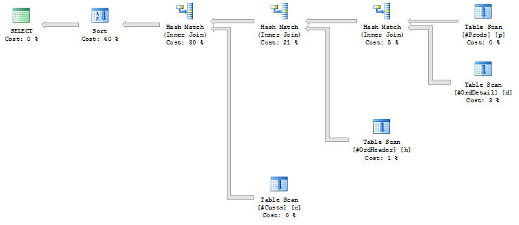
Take a look at the estimated plan of the first query without the ORDER BY:



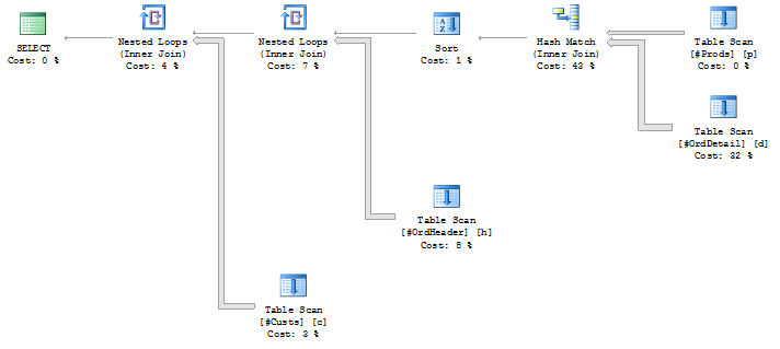
All the tables are JOINed with Hash Join operators. That makes sense, considering there are no primary keys or indexes defined. A Merge Join operator would require pre-sorted (i.e. indexed) data and a Nested Loops Join operator would do a SEEK on its inner input (which requires an index). So a Hash Join is the best (and really only) choice to JOIN the tables.

Now take a look at the estimated query plan with the ORDER BY added to the query:



Hmmm… The SORT operator is not at the top (i.e. left) of the tree but is instead placed further down the tree, with the JOIN of the #Prods and #OrdDetail tables. I guess that makes sense since we wanted the query to be ORDERed BY #Prods.ProductID. But the remaining Hash Joins got converted into Nested Loops Joins.

How come?

Notice the very thin arrow lines connecting the JOIN operators… in both plans above. The optimizer estimated that only 1 row (!!) would result from the JOIN of the #Prods and #OrdDetail tables. And because only 1 row is estimated, the optimizer figured it could just use a Nested Loops Join... because, hey, there’s only 1 row, and besides, a Nested Loops Join would preserve the order of the sorted rows, whereas a Hash Join may not.

But you and I know the reality of the situation is that there is not going to be only 1 row moving in the flow up the query tree… there are going to be 121,317 rows. The estimate is waaaay off.

Here’s what the Actual plan looks like for the 24-minute-long ORDER BY query.



Note the huge thick arrow lines now? They represent the actual number of rows processed. The Nested Loops Join to the #OrdHeader table performed a Table Scan of the 31465-row #OrdHeader table 121,317 times! So that resulted in 31465 * 121317 = 3,817,239,405 rows being processed. Similarly, a whopping 2,327,466,645 rows were processed out of the #Custs table. No wonder it took 24 minutes! Our friend Nora Nested-Loops must have been thoroughly exhausted at the end of this query!

So why the gross underestimation of the rows? Why did the optimizer figure that only 1 row would result in the JOIN of #Prods and #OrdDetail?

It’s those #$@*% multiple columns in the JOIN.

Take a look at how the estimates dramatically decrease as we add an additional predicate to the JOIN condition:

select p.ProductMainID as PID
      ,p.Name
      ,d.OrderQty
from #Prods p
join #OrdDetail d on p.ProductMainID=d.ProductMainID
/*
97783.6 Rows Estimated
*/
 
select p.ProductMainID as PID
      ,p.Name
      ,d.OrderQty
from #Prods p
join #OrdDetail d on p.ProductMainID=d.ProductMainID
                  and p.ProductSubID=d.ProductSubID 
/*
156.38 Rows Estimated
*/
 
select p.ProductMainID as PID
      ,p.Name
      ,d.OrderQty
from #Prods p
join #OrdDetail d on p.ProductMainID=d.ProductMainID
                  and p.ProductSubID=d.ProductSubID 
                  and p.ProductSubSubID=d.ProductSubSubID
/*
1 Row Estimated
*/

The optimizer does use statistics to attempt to estimate the row count, but the problem is that statistics are automatically created for each column individually… they are not created for the columns collectively. So when the optimizer sees two predicates in the JOIN condition (or three), it assumes the predicates are independent and therefore more and more selective.

In reality, that is not always the case in the real world. For example, let’s say you had a JOIN condition based on Make and Model and Year of automobile. If we’re trying to join on (’Toyota’, ’Prius’, 2010), the optimizer would make estimates based on how selective ‘Toyota’ is among all other Makes and on how selective ‘Prius’ is among all other Models (regardless of Make). A Prius is very selective among all Models… it’s one of hundreds. But a Prius is not that selective among Toyotas… it’s only one of about a dozen or so.

So this is what I was dealing with in this database… Lots of multi-column JOINs between Heaps which totally annihilate performance because of bad estimates.

In my case I was not able to create any indexes… Don’t ask me why… I don’t want to talk about it… It was essentially outside the scope of the project.

I mentioned earlier that statistics are automatically created on individual columns referenced in JOIN/WHERE conditions if they don’t exist already, but statistics for collective multiple columns are NOT automatically created. The great thing about indexes, though, is that a multi-column index WILL create collective multiple-column statistics, so the optimizer can make much better estimates when dealing with multiple-column predicates. So chalk that up as another really good reason to use indexes.

Actually, we can manually create collective multi-column statistics on our own like so, and upon doing so, the query is much much faster:

create statistics Stat_PID_Main_Sub_SubSub 
  on #Prods (ProductMainID,ProductSubID,ProductSubSubID)
create statistics Stat_PID_Main_Sub_SubSub 
  on #OrdDetail (ProductMainID,ProductSubID,ProductSubSubID)
go
 
select p.ProductMainID as PID
      ,p.Name
      ,d.OrderQty
      ,h.SalesOrderNumber
      ,h.OrderDate
      ,c.TerritoryID
from #Prods p
join #OrdDetail d on p.ProductMainID=d.ProductMainID
                  and p.ProductSubID=d.ProductSubID
                  and p.ProductSubSubID=d.ProductSubSubID
join #OrdHeader h on d.SalesOrderID=h.SalesOrderID
join #Custs c on h.CustomerID=c.CustomerID 
order by p.ProductMainID
/*
2910ms Duration
*/

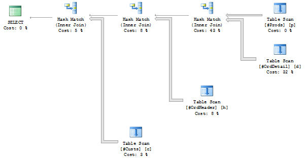
With those multi-column stats created, the estimated query plan now gets a very different shape:



Unfortunately, creating these multi-column statistics was also outside of the scope of my project with this client.

What was I to do?

I ended up going with hints… Not the greatest solution, but one that I could apply quickly to the code.

You may recall a blog post I wrote in August 2010 regarding Query Hints. In one example in that blog post, I introduced a hint to force the optimizer to use a Nested Loops Join rather than a Hash Join.

In this case, though, in dealing with the Heaps and their multi-column joins, I ended up doing the exact opposite… I introduced hints to force the use of Hash Joins rather than those pesky Nested Loops Joins.

So let’s change the query to the following, specifying a Hash Join for each Join:

select p.ProductMainID as PID
      ,p.Name
      ,d.OrderQty
      ,h.SalesOrderNumber
      ,h.OrderDate
      ,c.TerritoryID
from #Prods p
inner hash join #OrdDetail d on p.ProductMainID=d.ProductMainID
                             and p.ProductSubID=d.ProductSubID
                             and p.ProductSubSubID=d.ProductSubSubID
inner hash join #OrdHeader h on d.SalesOrderID=h.SalesOrderID
inner hash join #Custs c on h.CustomerID=c.CustomerID 
order by d.ProductMainID
/*
9701ms Duration
*/

That doesn’t run quite so quickly as the query that had the advantage of the multi-column stats, but 9.7 seconds is certainly better than 24 minutes!

The estimated query plan for the Hash Join Hint query looks like this:



It’s pretty much just like the plan for the non-ORDERBY query, except it has a SORT operator thrown in to execute at the top of the tree, after all the JOINs. When the optimizer sees Hash Join hints, it forces the query to be processed in order of how the JOINs are introduced in the query, so it first JOINs the #Prods and #OrdDetail, then the #OrdHeader, then the #Custs table.

By the way, for those of you who want to save typing, the same thing could be accomplished via the OPTION clause (instead of specifying individual JOIN hints), forcing the optimizer to use Hash Joins for every JOIN in the query:

select p.ProductMainID as PID
      ,p.Name
      ,d.OrderQty
      ,h.SalesOrderNumber
      ,h.OrderDate
      ,c.TerritoryID
from #Prods p
join #OrdDetail d on p.ProductMainID=d.ProductMainID
                  and p.ProductSubID=d.ProductSubID
                  and p.ProductSubSubID=d.ProductSubSubID
join #OrdHeader h on d.SalesOrderID=h.SalesOrderID
join #Custs c on h.CustomerID=c.CustomerID 
order by d.ProductMainID
option (hash join)
/*
9701ms Duration
*/

We could force the topology of the query plan to be just like the one that resulted from creating the statistics by rewriting the query like so:

select p.ProductMainID as PID
      ,p.Name
      ,d.OrderQty
      ,h.SalesOrderNumber
      ,h.OrderDate
      ,c.TerritoryID
from #Prods p
inner hash join (#OrdDetail d 
                 inner hash join (#OrdHeader h 
                                  inner hash join #Custs c 
                                             on h.CustomerID=c.CustomerID)
                            on d.SalesOrderID=h.SalesOrderID)
           on p.ProductMainID=d.ProductMainID
           and p.ProductSubID=d.ProductSubID
           and p.ProductSubSubID=d.ProductSubSubID                
order by d.ProductMainID
 

This forces the #Custs and #OrdHeader to JOIN first, then that result is JOINed to #OrdDetail, and then that result is finally JOINed to #Prods… just like the query plan that was able to use the multi-column stats. And it runs just as fast… 2.9 seconds.

However, that code is really difficult to read and figure out what’s going on. (It’s kinda cool, though, that we have the flexibility to write it that way, dontcha think?)

So we’ll have to settle for the 9.7 second query.

But thank goodness we can bring about these changes in behavior with the use of hints. They can certainly be a godsend when you don’t have any other options available to you.

Update Dec09,2010: Paul White wrote an excellent must-read follow-up to this article, giving some wonderful additional insights. If you’re not a regular reader of his blog, I must insist that you subscribe to it immediately. It’s a gold mine of terrific material.